EViews offers for financial institutions, corporations, government agencies, and academics access to powerful statistical, time series, forecasting, and modeling tools through an innovative, easy-to-use object-oriented interface.
With EViews you quickly and efficiently process your data, generate forecasts and high quality tables and graphs, allowing in this way an impressive visualization of your results.
In addition, EViews offers you an elegant and fast handling of time series of different granularity. EViews contains almost all established estimation models (LS, 2SLS, GLM, etc.), as well as all classical models (ARIMA, ARCH, GARCH, etc.) and opens up a variety of possibilities for simulating scenarios (Monte Carlo simulations, etc.).
Find out for yourself why EViews is the worldwide leader in Windows-based econometric software and the choice of those who demand the very best:
- An Intuitive, Easy-to-Use Interface
- Powerful Analytic Tools
- Sophisticated Data Management
- Presentation Quality Output
- Traditional Command Line and Programming Interface
See in the producer's video the new features for ecxample Bayesian Time-Varying Coefficient VAR:
Other improvements include:
- Enhanced ARDL and NARDL estimation
- Improved Pool Mean Group (PMG) estimation
- Difference-in-Difference estimation
- Bayesian Time-varying Coefficient VARs
- Enahanced VEC estimation
- Improved cointegration testing
- New ARDL and PMG diagnostics
- Panel Cluster Standard Errors
- Daily seasonal adjustment
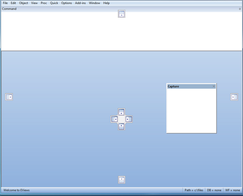
- Alternative graphical user interface
- Program debugging tools
- Run/program EViews in a Jupyter Notebook
- Graph improvements
- Table improvements
- Matrix language improvements
and more!
Key-Features of EViews:
- Estimates, forecasts and statistical analyses
- Equations estimation method for time series (AR, ARCH, GARCH etc. ), cross-tabs, etc.
- Hypothesis testing
- Stochastic Simulation (Monte Carlo Simulation etc.)
- Statistical and dynamic forecasts
- Data management via a powerful object-oriented interface: Automatic conversion of frequencies , support for Excel 2007 formats and ASCII import files from the FRED database, interaction with R and MATLAB programming, more than 4 million observations per series
- Smooth Threshold Regression (STR and STAR)
- Structural VAR restriction improvements
- New seasonal adjustment methods
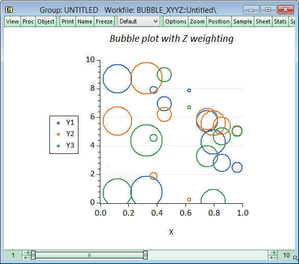
- New charting tools, including Bubble plots
- Automatic backup and data history system
- Improved R integration
- Connectivity with World Bank, Eurostat and others
- Saving as Tableau®
Recommended products
Stata BE
Stata SE
STATA MP
EViews
Forecasting within the Econometric Sector
EViews offers academic researchers, corporations, government agencies, and students access to powerful statistical, forecasting, and modeling tools through an innovative, easy-to-use object-oriented interface.
Its combination of power and ease-of-use make EViews the ideal package for anyone who works with time series, cross-section, or longitudinal data. With EViews, you can quickly and efficiently manage your data, perform econometric and statistical analysis, generate forecasts or model simulations, and produce high quality graphs and tables for publication or inclusion in other applications - just with mouse-clicks no complicated command language is needed!
Difference between EViews Standard and Enterprise Edition
EViews comes in two different editions: Standard and Enterprise. The Enterprise edition contains all the features of the Standard edition, but has some additional benefits:
- Database Connections
Whether you want to connect to a third party vendor, use ODBC to connect to a relational database, or use EViews’ Database Extension Interface (“EDX”) or EViews’ Database Object (“EDO”) Library to connect to your propriety data sources, EViews Enterprise is the tool for you!
- Third Party Vendors
With EViews Enterprise and an account with your data provider, you can seamlessly search, query, and retrieve data from third-party data sources such as Bloomberg databases, IHS databases, FactSet databases and many more.
EViews - Graphics
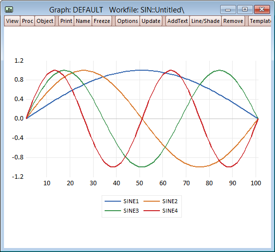
EViews supports a wide range of graph types including line graphs, bar graphs, pie charts, scatter diagrams, mixed line-bar graphs, high-low graphs, and scatterplots. A variety of options give you control over line types, color, border characteristics, headings, shading and scaling, including logarithmic scaling and dual scale graphs. Legends are automatically created and you can add labels in any scalable Windows fonts anywhere on your graph. Any number of graphs can be combined in a single graph for presentation. Customizing a graph is as simple as dragging graphic elements around the screen. Want to change the characteristics of a legend or a text label? Just click on it and your options are immediately presented in easy to understand dialogs. You can easily incorporate your customized graphs into other Windows applications using copy-and-paste, or by exporting Windows metafiles.
<
The IHS Global Link Model is the most comprehensive global macroeconomic model commercially available. With access through a unique desktop scenario application - the Economic Simulation Engine - IHS Global Link Model enables clients to generate macroeconomic scenarios and calculate their impact in minutes. Calculate in real-time global trends and prices of commodity, oil and gas, groceries, exchange rates and many more. All data of the IHS Global Link Model can be exported to the software EViews. Additionaly you get access to consulting via statistic- and analysis experts at IHS at any time.
Further Information:
- EViews-Homepage (IHS EViews)
- The manufacturer of EViews provides several Add-ins and Library Packages to increase the functionality of EViews.
Trainings for the Software EViews
STATCON not only offers professional statistical software solutions, we also offer professional trainings and consulting for those solutions so that you get the maximum out of your software! We offer simple trainings that will introduce you to the software and it's basic features but also more comprehensive trainings with deepth inside into specific functions of the software. Trainings are held as In-house and Off-site trainings. If you would like to attend a comfortable online-training, take a look at our webinars.
EViews - Introduction
This course introduces the basic statistical tools that are commonly used in econometris. The focus lies on linear regression analysis in the context of time series. At the same time EViews is introduced. Go to Article...
EViews - Scripting
This one day course is all about the EViews scripting language. Learn the typical aspects of programming language: loops, conditional statements, vectors and matrices. The training will cover database-access as well as graph customization and many real world examples. Go to Article...
EViews - Modelling: Complex Models
This two-day-course is an advanced training for the analysis of economic time series data. Vector-Autoregressive (VAR) and Vector-Error-Correction-Models (VEC) are part of the training as a special case of systems of equations. Final part of the training describes ways to model volatility of time series in form of Autoregressive Conditional Heteroscedasticity-models (ARCH, GARCH). Go to Article...
EViews Webinar - ARCH and GARCH
In this 3-hour online seminar the participant learns methods for modeling and forecasting volatility. These ARCH and GARCH models are discussed theoretically. Go to Article...
EViews Webinar (free) - Tips & Tricks
In this webinar we will introduce you to the installation and application of Add-Ins into EViews. Different Add-In's for the automatic ARIMA-model selection and the predictions for VAR-models are demonstrated. Go to Article...
EViews Software Updates & Patches
EViews offers a wide range of free minor updates and patches for their software. Those are available for the older versions of the software. Furthermore you can download several whitepapers, data and third party data interfaces.
EViews 13 System Requirements
|
CPU: |
Pentium or better |
|
|
Operating System: |
Windows 11 (64bit) |
Windows 10 (64bit) |
|
Memory: |
512 MB |
|
|
Disk Space: |
400 MB of available hard disk space for the EViews executable, supporting files, full documentation, and example files. |
Functions of the Software EViews
New Features in EViews 13:
EViews 13 features a wide range of exciting changes and improvements.
The following is an overview of the most important new features in Version 13.
EViews Interface and Programming
- Pane and Tab alternative user interface.
- Program Language Debugging.
- Jupyter Notebook Support.
- Program dependency tracking.
Data Handling
- Daily deasonal adjustment.
- Improved Excel writing engine.
- World Health Organisation connectivity
- Trading Economics connectivity
- National statistical bureaus connectivity
- Holiday function improvements
- Miscellaneous Improvements
New Graph, Table and Geomap Features
- Line and Shade Transparency
- Custom Data Labels
- High-low-median Colormap Presets
- Miscellaneous Improvements
Econometrics and Statistics
Estimation
- Non-linear ARDL Estimation
- Improved PMG Estimation
- Difference-in-Difference Estimation
- Improved VEC Estimation
- Bayesian Time-varying Coefficient Vector Autoregression
Testing and Diagnostics
- Cointegration Testing Enhancements
- ARDL Diagnostics
- Pool Mean Group / Panel ARDL Diagnostics
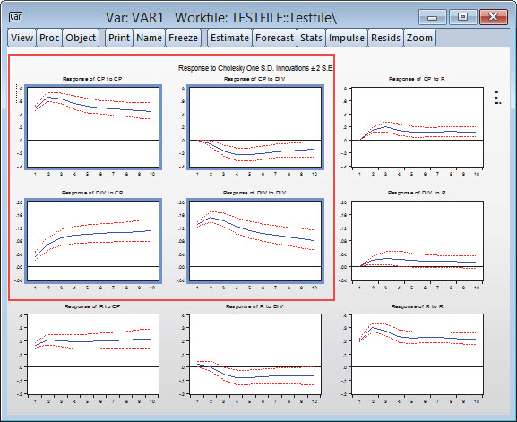
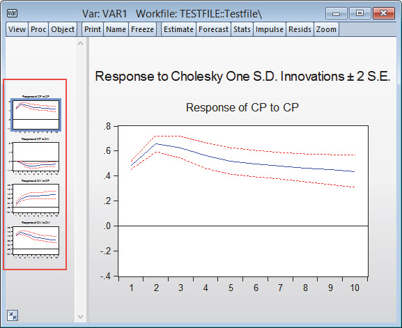
- Enhanced Impulse Response Display
Interesting Features in older EViews-Versions
EViews offers a multitude of exciting changes and improvements.
EViews Interface
Interactive command explorer to view all the applicable commands for an object and its documentation.
- Name and command auto-complete.
- Value-based spreadsheet and Geomap coloring.
Data Handling
- Integration with Python.
- Duplicates analysis.
- Split-observations high-to-low frequency conversion method.
- Interface to the following data sources
- Bureau of Economic Analysis (BEA).
- US Census.
- National Oceanic and Atmospheric Administration.
Graphs, Tables and Spools
- Geographic maps.
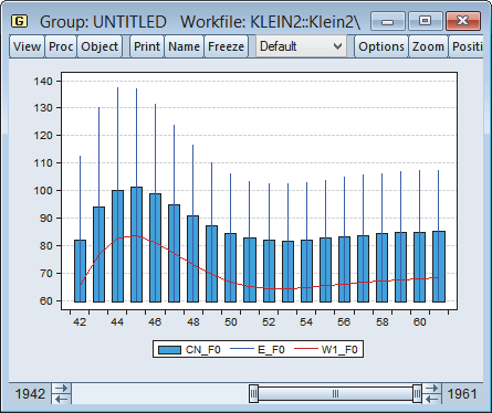
- Fan charts.
Econometrics and Statistics
Estimation
- Improved Bayesian VARs.
- Mixed frequency VARs.
- Switching VARs (Markov and simple).
- Elastic net and LASSO machine learning.
- Functional coefficient and localized regression.
- Additional cluster robust standard errors.
Testing and Diagnostics
- Seasonal unit root tests.
Interesting Features in older EViews-Versions
- Interface
Automatic and user-controlled workfile history, snapshot and backup system, Live statistics for
spreadsheet views, Support for long object names, Enhanced logging abilities.
- Data Handling
Improved integration with R, Attribute importing and exporting, Interface to World Bank data, Interface to United Nations data,
Interface to Eurostat data, Interface to European Central Bank data, Saving to Tableau®, Saving to JSON. - Graphs, Tables and Spools
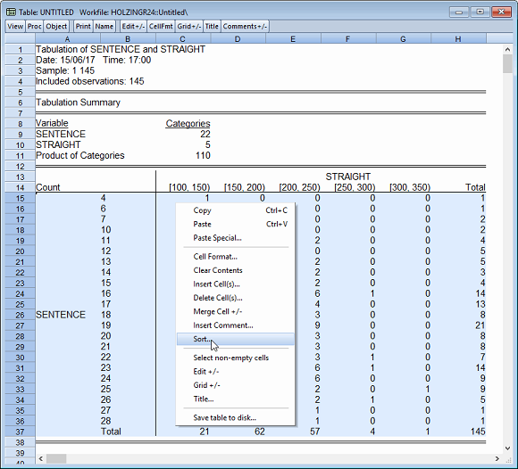
Bubble plots, Series updating in graphs, New default graph styles, Miscellaneous new graph options, Table sorting.
Econometrics and Statistics
- Computation
Season-trend decomposition (STL), MoveReg weekly seasonal adjustment, Special function computation.
-
Estamination
Smooth threshold regression (STR), Heteroskedasticity consistent robust stardard error options, Clustered stardard errors,
VARs with linear restrictions, Structural VAR restriction improvements, VAR historical decomposition,
Improved nonlinear forecasting, Additional autoregressive distributed lag (ARDL) tools.
- Testing and Diagnostics
VAR structural residuals, Improved VAR serial correlation testing, Model bounds checking. _____________________________________________________________________________________________________________________________
- MIDAS Estimation & Forecasting
Mixed Data Sampling is a method for estimating and forecasting models, the dependent variable is recorded at a lower frequency, as one or more of the independent variables (Mixed-frequency estamination). MIDAS enables estimates without aggregation and gives more accurate results. The EViews Workfiles allow easy organization of mixed frequency data and facilitates easy conversion from one frequency to another.
4 different MIDAS weighting schemes:- Step weights
- Almon/PDL weights
- Exponential Almon weights
- Beta weights
- FIML Estimation & Forecasting with Variance Restrictions
FIML estimator now has the ability to specify the form of the residual covariance matrix, which are given in estimates. This allows more efficient estimates. - Diebold-Marioano Test
Extension of the forecast comparison diagnostic tools. The Diebold-Mariano test allows comparison of two predictions from the same data set. - New Model Specifications
- Model Print View
A simple list of your model's scenarios (and their settings). - Modell Szenario Beschreibungen
Sie können Kommentare oder Beschreibungen zum Modell Szenario hinzufügen. Dies ermöglicht Ihnen einen besseren Überblick zu behalten. Es besteht auch die Möglichkeit zum Export der Beschreibungen zu Modellen innerhalb des Szenarios - Model Scenario Descriptions
Add descriptions to your model scenarios, and then export those descriptions to the solution series. - Equation Find
The Equation View of a model has a new Find button that lets you find an equation by name, by endogenous variable name or by exogenous variable name. - Model Protection
You can password protect your model so that users can only solve the model but not make changes to the model structure.
- Model Print View
- Group Members View
Graphical drag and drop user interface that displays the member series in the group and allows the user to alter these group members. - Group Object Preview
Allows users to preview a group object by displaying the group members along with a graph of group members. - Saving/Retrieving Program Variables
New functions to allow you to save and load program variables into text-ini files on disk:- Saveprgini: This allows the saving a program variable to an ini file.
- Loadprgini: This allows the retrieving of a program variable stored in a ini file.
Basic Data Handling
- Numeric, alphanumeric (string), and date series; value labels.
- Extensive library of operators and statistical, mathematical, date and string functions.
- Powerful language for expression handling and transforming existing data using operators and functions.
- Samples and sample objects facilitate processing on subsets of data.
- Support for complex data structures including regular dated data, irregular dated data, cross-section data with observation identifiers, dated, and undated panel data.
- Multi-page workfiles.
- EViews native, disk-based databases provide powerful query features and integration with EViews workfiles.
- Convert data between EViews and various spreadsheet, statistical, and database formats, including (but not limited to): Microsoft Access® and Excel® files (including .XSLX and .XLSM), Gauss
Dataset files, SAS® Transport files, SPSS native and portable files, Stata
files, Tableau®, raw formatted ASCII text or binary files, HTML, or ODBC databases
and queries (ODBC support is provided only in the Enterprise Edition). - OLE support for linking EViews output, including tables and graphs, to other packages, including Microsoft Excel®, Word® and Powerpoint®.
- OLEDB support for reading EViews workfiles and databases using OLEDB-aware clients or custom programs.
- Support for FRED® (Federal Reserve Economic Data), World Bank, and EuroStat databases. Enterprise Edition support for Global Insight DRIPro and DRIBase, Haver Analytics® DLX®, FAME, EcoWin, Bloomberg®, EIA®, CEIC®, Datastream®, FactSet®, and Moody’s Economy.com databases.
- The EViews Microsoft Excel® Add-in allows you to link or import data from EViews workfiles and databases from within Excel.
- Drag-and-drop support for reading data; simply drop files into EViews for automatic conversion and linking of foreign data and metadata into EViews workfile format.
- Powerful tools for creating new workfile pages from values and dates in existing series.
- Match merge, join, append, subset, resize, sort, and reshape (stack and unstack) workfiles.
- Easy-to-use automatic frequency conversion when copying or linking data between pages of different frequency.
- Frequency conversion and match merging support dynamic updating whenever underlying data change.
- Auto-updating formula series that are automatically recalculated whenever underlying data change.
- Easy-to-use frequency conversion: simply copy or link data between pages of different frequency.
- Tools for resampling and random number generation for simulation. Random number generation for 18 different distribution functions using three different random number generators.
- Support for cloud drive access, allowing you to open and save file directly to Dropbox, OneDrive, Google Drive and Box accounts.
Time Series Data Handling
- Integrated support for handling dates and time series data (both regular and irregular).
- Support for common regular frequency data (Annual, Semi-annual, Quarterly, Monthly, Bimonthly, Fortnight, Ten-day, Weekly, Daily - 5 day week, Daily - 7 day week).
- Support for high-frequency (intraday) data, allowing for hours, minutes, and seconds frequencies. In addition, there are a number of less commonly encountered regular frequencies, including Multi-year, Bimonthly, Fortnight, Ten-Day, and Daily with an arbitrary range of days of the week.
- Specialized time series functions and operators: lags, differences, log-differences, moving averages, etc.
- Frequency conversion: various high-to-low and low-to-high methods.
- Exponential smoothing: single, double, Holt-Winters, and ETS smoothing.
- Built-in tools for whitening regression.
- Hodrick-Prescott filtering.
- Band-pass (frequency) filtering: Baxter-King, Christiano-Fitzgerald fixed length and full sample asymmetric filters.
- Seasonal adjustment: Census X-13, STL Decomposition, MoveReg, X-12-ARIMA, Tramo/Seats, moving average.
- Interpolation to fill in missing values within a series: Linear, Log-Linear, Catmull-Rom Spline, Cardinal Spline.
Statistics
Basic
- Basic data summaries; by-group summaries.
- Tests of equality: t-tests, ANOVA (balanced and unbalanced, with or without heteroskedastic variances.), Wilcoxon, Mann-Whitney, Median Chi-square, Kruskal-Wallis, van der Waerden, F-test, Siegel-Tukey, Bartlett, Levene, Brown-Forsythe.
- One-way tabulation; cross-tabulation with measures of association (Phi Coefficient, Cramer’s V, Contingency Coefficient) and independence testing (Pearson Chi-Square, Likelihood Ratio G^2).
- Covariance and correlation analysis including Pearson, Spearman rank-order, Kendall’s tau-a and tau-b and partial analysis.
- Principal components analysis including scree plots, biplots and loading plots, and weighted component score calculations.
- Factor analysis allowing computation of measures of association (including covariance and correlation), uniqueness estimates, factor loading estimates and factor scores, as well as performing estimation diagnostics and factor rotation using one of over 30 different orthogonal and oblique methods.
- Empirical Distribution Function (EDF) Tests for the Normal, Exponential, Extreme value, Logistic, Chi-square, Weibull, or Gamma distributions (Kolmogorov-Smirnov, Lilliefors, Cramer-von Mises, Anderson-Darling, Watson).
- Histograms, Frequency Polygons, Edge Frequency Polygons, Average Shifted Histograms, CDF-survivor-quantile, Quantile-Quantile, kernel density, fitted theoretical distributions, boxplots.
- Scatterplots with parametric and non-parametric regression lines (LOWESS, local polynomial), kernel regression (Nadaraya-Watson, local linear, local polynomial)., or confidence ellipses.
Time Series
- Autocorrelation, partial autocorrelation, cross-correlation, Q-statistics.
- Granger causality tests, including panel Granger causality.
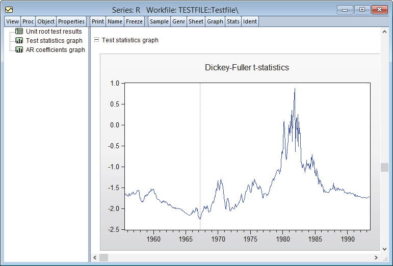
- Unit root tests: Augmented Dickey-Fuller, GLS transformed Dickey-Fuller, Phillips-Perron, KPSS, Eliot-Richardson-Stock Point Optimal, Ng-Perron, as well as tests for unit roots with breakpoints.
- Cointegration tests: Johansen, Engle-Granger, Phillips-Ouliaris, Park added variables, and Hansen stability.
- Independence tests: Brock, Dechert, Scheinkman and LeBaron
- Variance ratio tests: Lo and MacKinlay, Kim wild bootstrap, Wright's rank, rank-score and sign-tests. Wald and multiple comparison variance ratio tests (Richardson and Smith, Chow and Denning).
- Long-run variance and covariance calculation: symmetric or or one-sided long-run covariances using nonparametric kernel (Newey-West 1987, Andrews 1991), parametric VARHAC (Den Haan and Levin 1997), and prewhitened kernel (Andrews and Monahan 1992) methods. In addition, EViews supports Andrews (1991) and Newey-West (1994) automatic bandwidth selection methods for kernel estimators, and information criteria based lag length selection methods for VARHAC and prewhitening estimation.
Panel and Pool
- By-group and by-period statistics and testing.
- Unit root tests: Levin-Lin-Chu, Breitung, Im-Pesaran-Shin, Fisher, Hadri.
- Cointegration tests: Pedroni, Kao, Maddala and Wu.
- Panel within series covariances and principal components.
- Dumitrescu-Hurlin (2012) panel causality tests.
- Cross-section dependence tests.
Estimation
Regression
- Linear and nonlinear ordinary least squares (multiple regression).
- Linear regression with PDLs on any number of independent variables.
- Robust regression.
- Analytic derivatives for nonlinear estimation.
- Weighted least squares.
- White and other heteroskedasticity consistent, and Newey-West robust standard errors. HAC standard errors may be computed using nonparametric kernel, parametric VARHAC, and prewhitened kernel methods, and allow for Andrews and Newey-West automatic bandwidth selection methods for kernel estimators, and information criteria based lag length selection methods for VARHAC and prewhitening estimation.
- Clustered standard errors.
- Linear quantile regression and least absolute deviations (LAD), including both Huber’s Sandwich and bootstrapping covariance calculations.
- Stepwise regression with seven different selection procedures.
- Threshold regression including TAR and SETAR, and smooth threshold regression including STAR.
- ARDL estimation, including the Bounds Test approach to cointegration.
ARMA and ARMAX
- Linear models with autoregressive moving average, seasonal autoregressive, and seasonal moving average errors.
- Nonlinear models with AR and SAR specifications.
- Estimation using the backcasting method of Box and Jenkins, conditional least squares, ML or GLS.
- Fractionally integrated ARFIMA models.
Instrumental Variables and GMM
- Linear and nonlinear two-stage least squares/instrumental variables (2SLS/IV) and Generalized Method of Moments (GMM) estimation.
- Linear and nonlinear 2SLS/IV estimation with AR and SAR errors.
- Limited Information Maximum Likelihood (LIML) and K-class estimation.
- Wide range of GMM weighting matrix specifications (White, HAC, User-provided) with control over weight matrix iteration.
- GMM estimation options include continuously updating estimation (CUE), and a host of new standard error options, including Windmeijer standard errors.
- IV/GMM specific diagnostics include Instrument Orthogonality Test, a Regressor Endogeneity Test, a Weak Instrument Test, and a GMM specific breakpoint test.
ARCH/GARCH
- GARCH(p,q), EGARCH, TARCH, Component GARCH, Power ARCH, Integrated GARCH.
- The linear or nonlinear mean equation may include ARCH and ARMA terms; both the mean and variance equations allow for exogenous variables.
- Normal, Student’s t, and Generalized Error Distributions.
- Bollerslev-Wooldridge robust standard errors.
- In- and out-of sample forecasts of the conditional variance and mean, and permanent components.
Limited Dependent Variable Models
- Binary Logit, Probit, and Gompit (Extreme Value).
- Ordered Logit, Probit, and Gompit (Extreme Value).
- Censored and truncated models with normal, logistic, and extreme value errors (Tobit, etc.).
- Count models with Poisson, negative binomial, and quasi-maximum likelihood (QML) specifications.
- Heckman Selection models.
- Huber/White robust standard errors.
- Count models support generalized linear model or QML standard errors.
- Hosmer-Lemeshow and Andrews Goodness-of-Fit testing for binary models.
- Easily save results (including generalized residuals and gradients) to new EViews objects for further analysis.
- General GLM estimation engine may be used to estimate several of these models, with the option to include robust covariances.
Panel Data/Pooled Time Series, Cross-Sectional Data
- Linear and nonlinear estimation with additive cross-section and period fixed or random effects.
- Choice of quadratic unbiased estimators (QUEs) for component variances in random effects models: Swamy-Arora, Wallace-Hussain, Wansbeek-Kapteyn.
- 2SLS/IV estimation with cross-section and period fixed or random effects.
- Estimation with AR errors using nonlinear least squares on a transformed specification
- Generalized least squares, generalized 2SLS/IV estimation, GMM estimation allowing for cross-section or period heteroskedastic and correlated specifications.
- Linear dynamic panel data estimation using first differences or orthogonal deviations with period-specific predetermined instruments (Arellano-Bond).
- Panel serial correlation tests (Arellano-Bond).
- Robust standard error calculations include seven types of robust White and Panel-corrected standard errors (PCSE).
- Testing of coefficient restrictions, omitted and redundant variables, Hausman test for correlated random effects.
- Panel unit root tests: Levin-Lin-Chu, Breitung, Im-Pesaran-Shin, Fisher-type tests using ADF and PP tests (Maddala-Wu, Choi), Hadri.
- Panel cointegration estimation: Fully Modified OLS (FMOLS, Pedroni 2000) or Dynamic Ordinary Least Squares (DOLS, Kao and Chaing 2000, Mark and Sul 2003).
- Pooled Mean Group (PMG) estimation.
Generalized Linear Models
- Normal, Poisson, Binomial, Negative Binomial, Gamma, Inverse Gaussian, Exponential Mena, Power Mean, Binomial Squared families.
- Identity, log, log-complement, logit, probit, log-log, complimentary log-log, inverse, power, power odds ratio, Box-Cox, Box-Cox odds ratio link functions.
- Prior variance and frequency weighting.
- Fixed, Pearson Chi-Sq, deviance, and user-specified dispersion specifications. Support for QML estimation and testing.
- Quadratic Hill Climbing, Newton-Raphson, IRLS - Fisher Scoring, and BHHH estimation algorithms.
- Ordinary coefficient covariances computed using expected or observed Hessian or the outer product of the gradients. Robust covariance estimates using GLM, HAC, or Huber/White methods.
Single Equation Cointegrating Regression
- Support for three fully efficient estimation methods, Fully Modified OLS (Phillips and Hansen 1992), Canonical Cointegrating Regression (Park 1992), and Dynamic OLS (Saikkonen 1992, Stock and Watson 1993
- Engle and Granger (1987) and Phillips and Ouliaris (1990) residual-based tests, Hansen's (1992b) instability test, and Park's (1992) added variables test.
- Flexible specification of the trend and deterministic regressors in the equation and cointegrating regressors specification.
- Fully featured estimation of long-run variances for FMOLS and CCR.
- Automatic or fixed lag selection for DOLS lags and leads and for long-run variance whitening regression.
- Rescaled OLS and robust standard error calculations for DOLS.
User-specified Maximum Likelihood
- Use standard EViews series expressions to describe the log likelihood contributions.
- Examples for multinomial and conditional logit, Box-Cox transformation models, disequilibrium switching models, probit models with heteroskedastic errors, nested logit, Heckman sample selection, and Weibull hazard models.
Systems of Equations
Basic
- Linear and nonlinear estimation.
- Least squares, 2SLS, equation weighted estimation, Seemingly Unrelated Regression, and Three-Stage Least Squares.
- GMM with White and HAC weighting matrices.
- AR estimation using nonlinear least squares on a transformed specification.
- Full Information Maximum Likelihood (FIML).
VAR/VEC
- Estimate structural factorizations in VARs by imposing short- or long-run restrictions, or both.
- Bayesian VARs.
- Impulse response functions in various tabular and graphical formats with standard errors calculated analytically or by Monte Carlo methods.
- Impulse response shocks computed from Cholesky factorization, one-unit or one-standard deviation residuals (ignoring correlations), generalized impulses, structural factorization, or a user-specified vector/matrix form.
- Historical decomposition of standard VAR models.
- Impose and test linear restrictions on the cointegrating relations and/or adjustment coefficients in VEC models.
- View or generate cointegrating relations from estimated VEC models.
- Extensive diagnostics including: Granger causality tests, joint lag exclusion tests, lag length criteria evaluation, correlograms, autocorrelation, normality and heteroskedasticity testing, cointegration testing, other multivariate diagnostics.
Multivariate ARCH
- Conditional Constant Correlation (p,q), Diagonal VECH (p,q), Diagonal BEKK (p,q), with asymmetric terms.
- Extensive parameterization choice for the Diagonal VECH's coefficient matrix.
- Exogenous variables allowed in the mean and variance equations; nonlinear and AR terms allowed in the mean equations.
- Bollerslev-Wooldridge robust standard errors.
- Normal or Student's t multivariate error distribution
- A choice of analytic or (fast or slow) numeric derivatives. (Analytics derivatives not available for some complex models.)
- Generate covariance, variance, or correlation in various tabular and graphical formats from estimated ARCH models.
State Space
- Kalman filter algorithm for estimating user-specified single- and multiequation structural models.
- Exogenous variables in the state equation and fully parameterized variance specifications.
- Generate one-step ahead, filtered, or smoothed signals, states, and errors.
- Examples include time-varying parameter, multivariate ARMA, and quasilikelihood stochastic volatility models.
Testing and Evaluation
- Actual, fitted, residual plots.
- Wald tests for linear and nonlinear coefficient restrictions; confidence ellipses showing the joint confidence region of any two functions of estimated parameters.
- Other coefficient diagnostics: standardized coefficients and coefficient elasticities, confidence intervals, variance inflation factors, coefficient variance decompositions.
- Omitted and redundant variables LR tests, residual and squared residual correlograms and Q-statistics, residual serial correlation and ARCH LM tests.
- White, Breusch-Pagan, Godfrey, Harvey and Glejser heteroskedasticity tests.
- Stability diagnostics: Chow breakpoint and forecast tests, Quandt-Andrews unknown breakpoint test, Bai-Perron breakpoint tests, Ramsey RESET tests, OLS recursive estimation, influence statistics, leverage plots.
- ARMA equation diagnostics: graphs or tables of the inverse roots of the AR and/or MA characteristic polynomial, compare the theoretical (estimated) autocorrelation pattern with the actual correlation pattern for the structural residuals, display the ARMA impulse response to an innovation shock and the ARMA frequency spectrum.
- Easily save results (coefficients, coefficient covariance matrices, residuals, gradients, etc.) to EViews objects for further analysis.
See also Estimation and Systems of Equations for additional specialized testing procedures.
Forecasting and Simulation
- In- or out-of-sample static or dynamic forecasting from estimated equation objects with calculation of the standard error of the forecast.
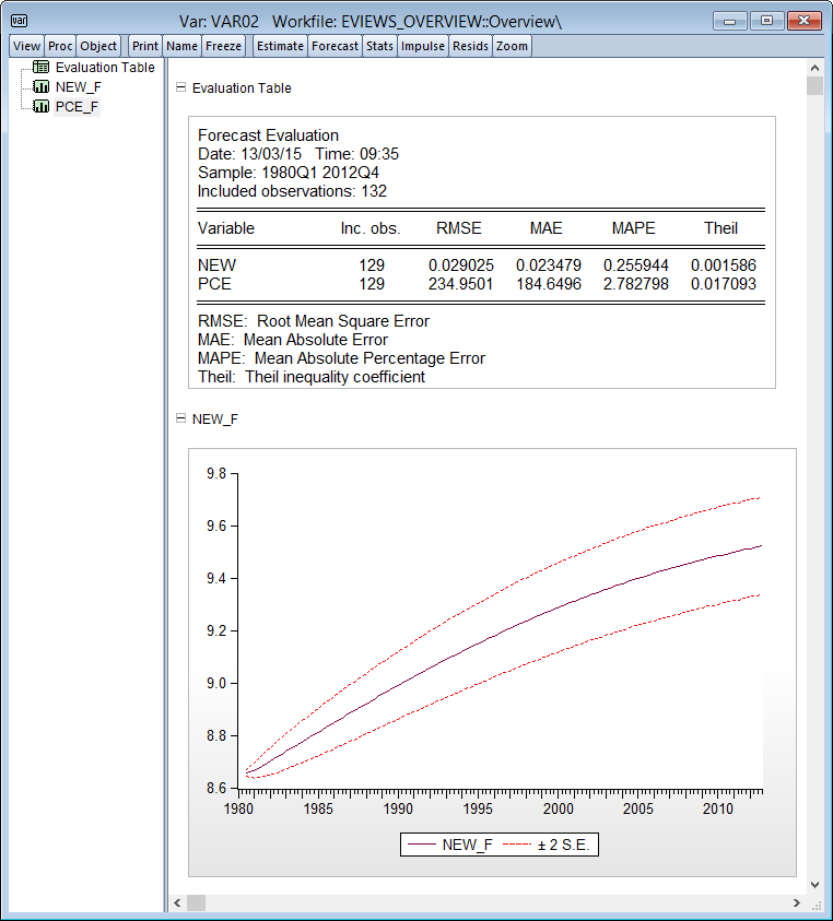
- Forecast graphs and in-sample forecast evaluation: RMSE, MAE, MAPE, Theil Inequality Coefficient and proportions
- State-of-the-art model building tools for multiple equation forecasting and multivariate simulation.
- Model equations may be entered in text or as links for automatic updating on re-estimation.
- Display dependency structure or endogenous and exogenous variables of your equations.
- Gauss-Seidel, Broyden and Newton model solvers for non-stochastic and stochastic simulation. Non-stochastic forward solution solve for model consistent expectations. Stochasitc simulation can use bootstrapped residuals.
- Solve control problems so that endogenous variable achieves a user-specified target.
- Sophisticated equation normalization, add factor and override support.
- Manage and compare multiple solution scenarios involving various sets of assumptions.
- Built-in model views and procedures display simulation results in graphical or tabular form.
Graphs and Tables
- Line, dot plot, area, bar, spike, seasonal, pie, xy-line, scatterplots, bubbleplots, boxplots, error bar, high-low-open-close, and area band.
- Powerful, easy-to-use categorical and summary graphs.
- Auto-updating graphs which update as underlying data change.
- Observation info and value display when you hover the cursor over a point in the graph.
- Histograms, average shifted historgrams, frequency polyons, edge frequency polygons, boxplots, kernel density, fitted theoretical distributions, boxplots, CDF, survivor, quantile, quantile-quantile.
- Scatterplots with any combination parametric and nonparametric kernel (Nadaraya-Watson, local linear, local polynomial) and nearest neighbor (LOWESS) regression lines, or confidence ellipses.
- Interactive point-and-click or command-based customization.
- Extensive customization of graph background, frame, legends, axes, scaling, lines, symbols, text, shading, fading, with improved graph template features.
- Table customization with control over cell font face, size, and color, cell background color and borders, merging, and annotation.
- Copy-and-paste graphs into other Windows applications, or save graphs as Windows regular or enhanced metafiles, encapsulated PostScript files, bitmaps, GIFs, PNGs or JPGs.
- Copy-and-paste tables to another application or save to an RTF, HTML, LaTeX, PDF, or text file.
- Manage graphs and tables together in a spool object that lets you display multiple results and analyses in one object
Commands and Programming
- Object-oriented command language provides access to menu items.
- Batch execution of commands in program files.
- Looping and condition branching, subroutine, and macro processing.
- String and string vector objects for string processing. Extensive library of string and string list functions.
- Extensive matrix support: matrix manipulation, multiplication, inversion, Kronecker products, eigenvalue solution, and singular value decomposition.
External Interface and Add-Ins
- EViews COM automation server support so that external programs or scripts can launch or control EViews, transfer data, and execute EViews commands.
- EViews offers COM Automation client support application for MATLAB® and R so that EViews may be used to launch or control the application, transfer data, or execute commands.
- The EViews Microsoft Excel® Add-in offers a simple interface for fetching and linking from within Microsoft Excel® (2000 and later) to series and matrix objects stored in EViews workfiles and databases.
- The EViews Add-ins infrastructure offers seamless access to user-defined programs using the standard EViews command, menu, and object interface.
- Download and install predefined Add-ins from the EViews website.


