

Design Expert for Mac and Windows

Design-Expert offers you the latest technology for multi-factorial data analysis and design of experiments in a very user-friendly environment. Design Expert walks you through the classic stages of the screening, optimization (RSM) and validation and provides the flexibility to map complex tasks in a “simple” experimental design. Design Expert thus allows you to save time and costs of developing new products while achieving the best process conditions.
This includes so called hard-to-change factors (for split-plot designs ) and optimization of chemical formulations or mixture designs as well as combined designs which handle mixture and process factors in a single experiment.
Design-Expert provides the rotatable 3D plot. It helps you to visualize so-called response surfaces. The optimum is reached via the numerical optimization function. There, the optimal factor settings are determined simultaneously. The optimization platform controls mulitivariate optimization to allow, for example, multiple target values being simultaneously optimized. Thus, conflicts conflicts between target variables can be solved.
Arguments for Design Expert:
- Rotatable 3D graphics, interactive contour diagrams (isolines), best ternary representation,
- All classical experimental designs, d-optimal for screening and i-optimal for RSM,
- Latest split-plot designs and definitive screening designs,
- Best optimizing function (multiple target variables and optimizing with respect to factor settings),
- Fitted function exported as a formula to Excel
- Error propagation (propagation of error ) helps you to find robust settings
- Indispensable for formulation optimizing
Recommended products

Design Expert - Mixture Designs

Design Expert - Introduction

Design Expert - Process Optimization
Design Expert
Best of breed in Design of Experiments!
Optimize your product or process with Design of Experiments (DOE). Design Expert offers features you will not find anywhere else in an incredibly easy-to-use format. This powerful program is a must for anyone wanting to improve a process or a product. With Design-Expert you can screen for vital factors, locate ideal process settings to achieve peak performance and discover your optimal product formulations. Interactive 2-D graphics support use of your mouse to drag contours or set flags that display coordinates and predicted responses. Rotatable 3-D plots make response visualization easy.
Developed with constant focus on the Usability
With annotated statistical analysis and an extensive context-sensitive help system, you can easily interpret the outputs. Furthermore the Design Wizards supports users who are new to the software or are just unsure where to start with their experiment. A short series of questions will guide them to the proper design.
Comprehensive and fully developed Functions
With the powerful optimization features in Design-Expert, you can maximize desirability for dozens of responses simultaneously. There are also unique tools for generating and graphing propagation of error (POE), thus allowing you to achieve six-sigma objectives for reducing variation. Maximize, minimize or hit targets with factor levels set to give you robust results.
Tremendous Variety of Designs Meet All Your Experimental Needs
- Standard two-level full and fractional factorials (up to 512 runs) for testing up to 21 factors simultaneously, now also with minimum-aberration blocking choices
- General (multilevel) factorial designs using factors with mixed levels
- Taguchi orthogonal arrays
- High-resolution irregular fractions, such as 4 factors in 12 runs
- Placket-Burman designs for 11, 19, 23, 27 or 31 factors in 12, 20, 24, 28, 32 or 64 runs respectively
- “Min-Run Res IV” (two-level factorial) designs for 5 to 50 factors: Screen main effects with maximum efficiency in terms of experimental runs.
- Response Surface Method (RSM) designs, including central composite (small, face-centered, etc.), Box- Behnken (3-level), hybrid and D-Optimal
- Mixture designs, such as simplex-lattice, simplex-centroid screening (for up to 24 components) and D-optimal
- Combined mixture and process designs (mix your cake and bake it, too!)
- Ability to graph any two columns of data on the XY graph (this is a great way to view a blocked effect)
- Easy-to-use automatic or manual model reduction
- Ability to easily analyze designs with botched or missing data
Enjoy Incredible Flexibility in Design Modification
- Define your own generators for fractional factorial designs
- Impose linear multivariable constraints on RSM or mixture designs
- Add categorical factors to RSM, mixture or combined designs
- Create a factorial candidate set for RSM designs when only specific factor levels are available
- Ignore a row of data while preserving the numbers
Build Confidence with Statistical Analysis of Data
- If your model is aliased, a warning will pop up prior to viewing the ANOVA for two-level fractional factorials, allowing you to make substitutions for aliased effects
- Select optional annotated views for assistance interpreting the ANOVA
- Inspect F-test values on individual model terms and confidence intervals on coefficients
- Automatically select effects using Lenth's criteria or probability values
- Take advantage of new user preferences, for example, make a global change in the significance threshold (0.05 by default vs. 0.01 and 0.1)
Take Advantage of Powerful Tools for Response Modeling
- Change models from RSM to factorial and back and from Scheffe (mixture) to slack (during design building and at model selection)
- Add integer power terms to the model, for example, quartic
- Select terms for model, error, or to be ignored (allows analysis of split-plot and nested designs)
Simplify Interpretation with Terrific Graphics
- A quick summary of the design type as well as factor, response and model information is available by clicking on the design status node
- Discover significant effects at a glance with half-normal or normal probability plots, made easier by including points representing estimates of pure error (if available from your design)
- See the Box-Cox plot for advice on the best response transformation
- View a complete array of diagnostic graphs to check statistical assumptions and detect possible outliers (bonus feature: predicted-versus-actual graphs with a 45º line)
- Graph alternative aliased interactions
- See the effects plot in the original scale after transforming the response
- Observe variation in predictions by viewing the least significant difference (LSD) bars on the model graphs
- Poorly predicted regions on contour maps are shaded to give you confidence in your predictions
- Slice your contour plots using a simple slide bar (and see actual design points when they're on a slice!)
- Set flags to reveal the predicted response at any location
- Drag 2-D contours using your mouse
- Rotate 3-D graphics and see projected 2-D contours
- Edit colors, text and more to produce professional reports
- See all effects on one graph with trace and perturbation plots
- Plot the standard error of your design on any graph type (contour, 3-D, etc.)
- Maximize, minimize or target specific levels for both responses and factors
- Set weight and importance levels to prioritize responses for desirability
- Choose 2-D contour, 3-D surface, histogram or ramp desirability graphs
- Include categorical factors
- Set factors at constant levels
- Add equation-only responses, such as cost, to the optimization process
- Look at the overlay plot to view constraints on your process or formulation
- Predict responses at any set of conditions (including confidence levels)
- Discover optimal process conditions or formulations

Achieve "Six-Sigma" Goals
- Explore propagation of error (POE) for mixtures, crossed designs and transformed responses, as well as RSM
- For purposes of POE, enter your own response standard deviation or set it at zero
Further Information
Design Expert - Trial
A Design Expert trial version is available for download directly from Stat-Ease, the manufacturing company of Design Expert. Take advantage of the opportunity to test the newest version of Design Expert. Design Expert trial comes at no costs and is valid for 14 days. During download you will be requested to register at Stat-Ease: https://www.statease.com/dx-
Tutorials for Design Expert
Statease provides various tutorials, guides and manuals for the latest Design Expert on their website. For reading these documents you need the Acrobat Reader from Adobe. https://www.statease.com/docs/latest/tutorials/
System Requirements for the Software Design Expert
| Windows | Mac | |
| Operating System | Windows 8, 8.1, 10, 11 | macOS 10.12 and higher |
| Min. CPU | 1 GHz | 1 GHz |
| Min. RAM | 2 GB | 2 GB |
| Disk Space | 250 MB | 250 MB |
| Further Requirement | (1024x768 or higher) | 1024x768 |
New Functions in Design Expert
Multi-Graph-View
Seeing effects from input variables side by side shouts out their relative impacts.

All Responses Choice
Compare side by side the overall desirability with the individual optimum results so you get the complete view from the peak of performance.

Design Wizard
The Design Wizard provides guidance for less sophisticated users: If you are not sure where to start with your experiment, follow through with this short series of questions to get an answer.

Expanded Undo/Redo Option
Expanded the Undo/Redo Option with a viewer toolbox, showing you the changes when using these options.

New Designs
Various new designs have been added to Design Expert:
- Blocking for Definitive Screening Designs (DSDs): these newly-invented designs are now even better with the option to break them up into blocks.
- Restricted Randomization Central Composite Designs (CCD): Convert this tried and true response surface method (RSM) design into a split plot so it can deal with hard-to-change factors.
- Optimal split plots for Response Surface and Combined (mixture-process) designs: They make it far easier as a practical matter to experiment when some factors cannot be easily randomized
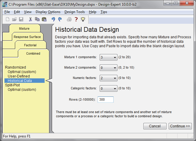
- Historical data choice for Combined designs: Take advantage of all the tools in Design-Expert— evaluation, model fitting, statistics, diagnostics, graphing and numerical optimization—to see if a sweet spot can be found in your collection of happenstance data, even if it includes both process factors and mixture components.
- Power and sample size calculator for binomial responses during build: Design an experiment with sufficient runs to be fairly certain that you will not overlook an important discovery. That is not all! Several more design build

Modeling tools supercharged
- Definitive Screening Designs (DSD) moved to the Response Surface tab where they can be analyzed as a supersaturated matrix for quadratic modeling
- AICc, BIC and Adjusted R-squared criteria in algorithmic selection
- Automatic Model Selection tool for choosing Criterion and Selection method

Other New Features
Technical Improvements
- 64-bit version now available: Take full advantage of the technology built into your CPU for faster performance for statistical calculations, rendering of graphics and so forth.
- Math engine retooled for far-faster computations.
- Optimal builds now run in parallel making them 3 to 17 times faster!
- Designs no longer limited to 32K runs.
Graphs
- Interactive LSD (least significant difference) bars
- Improved flexibility in sizing and placement of flags on graphs
- Show ignored values on Predicted vs Actual graphs
- Ability to turn off the factor names on plots
- Select a point after adding a comment on a graph
Interface
- Smoother scrolling of reports and spreadsheets
- Enhanced copy-paste for equations
- Improved export to Excel, Word and Powerpoint
- Support for different decimal point characters (localization)
- LOESS Tool for Fit line in Graph Columns
- Improved Graph Columns correlation grid tool with more intuitive layout
- Enhanced constraint tool with simplified result equations and a clear button
- Remember and restore position in design layout when returning to view
- Insert runs both before and after the selected run
- Double-click to resize reports
- Splash screen upon start (replaces About Box)
- Watermark added to example pictures on the transformation screen
- Better handling of progress bars including threading
Designs
- New expanded and redesigned Evaluation Report for split-plot designs
- Run column “Reorder as currently displayed” option for split-plot designs
- Column sort from View menu for Design Layout
- Variance ratio displayed on the power response-entry screen for split-plots
Modeling
- Select by Degree option prioritizes the criteria comparisons by term order
- Model Selection Log in Automatic Model Selection and in ANOVA
- Likelihood ratio p-values for split-plot designs
- Forward selection for REML/ML analysis
- Aliases reported and selectable in Effects List (makes Alias List unnecessary)
- Curvature term removed for DSDs (or other SDs that model squared terms)
Analysis
- Option to ignore groups for split-plot designs
- Equations section on the split-plot ANOVA
- Split-plot designs analyzed using either Maximum Likelihood (ML) or REML
- Tolerance Intervals for predictions in split-plot designs
- VIFs in split-plot ANOVA
- Adjustable REML/ML stopping rule and maximum iterations
- Negative variances excluded when calculating REML/ML
- Variance components in mixed-models are zeroed out below a threshold
- Improved computation of R2 in split-plot designs
- Block variance no longer included when calculating LSD values
- Option to choose between one-sided and two-sided tests for intervals
- New toolbox to view the V-matrix used in Mixed Model calculations
Diagnostics
- Box-Cox plot for mixed models, e.g., split plots
- Externally studentized residuals and influence graphs for mixed models (Cook's Distance, DFFITS, Covariance Trace and Covariance Ratio)
- Limit lines on diagnostic graphs are labeled
- Color by Group in the Residual vs Factor diagnostic graph
- Control limit default values for DFFITs and DFBETAs with the option not to display them on the graph
- Better footnoting in the Diagnostics Report