Loglineare Varianz Modell
Nichtkonstante Varianz in den Residuen einer Regressionsanalyse muss nicht immer ein Problem sein. Zwar nimmt die Methode der kleinsten Quadrate Homoskedastizität (=konstante Varianz) an, allerdings gibt es noch flexiblere Methoden, die ohne diese Annahme auskommen. Loglinear Variance Models erlauben nicht nur korrekte Signifikanzaussagen bei vorliegen von Heteroskedastie. Mit dieser, hier vorgestellten Modellklasse kann man gleichzeitig etwas über die technischen Ursachen erhöhter Streuung lernen.
Einleitung und Beispiel
Werfen wir einen Blick auf die folgenden Daten:

Es liegt ein teilfaktorieller Versuchsplan vor, der von der National Railway Corporation of Japan durchgeführt wurde [beschrieben in: G.Smyth 2002, Original: Taguchi & Wu 1980]. Damit wurde der Einfluß von neun Faktoren auf die Reißfestigkeit von Schweißnähten untersucht. Dazu wurden 16 Experimente durchgeführt. Eine einfache Analyse mittles der Screening-Plattform in JMP deutet darauf hin, dass die Faktoren [C] Material und [B] Drying wichtig sind. [F] Opening und [A] Rods könnten durchaus auch eine Rolle spielen.
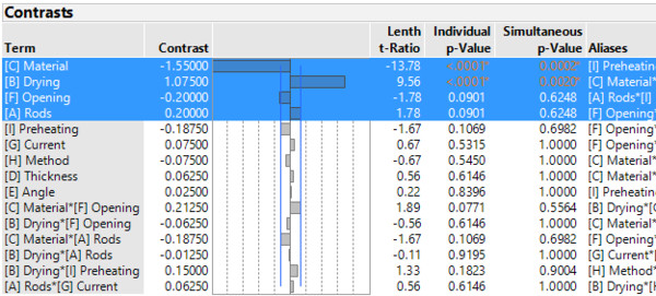
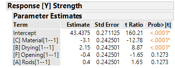
In den Ergebnissen der (OLS) Regressionsanalyse wird der Einfluß von [C] und [B] auf die Reißfestigkeit bestätigt. Auch wenn [F] und [A] keinen signifikanten Einfluß aufweisen, könnte man sich vorstellen diese Faktoren dennoch näher zu untersuchen. Wie immer muss Anwendungswissen ausschlaggebend für die Modellbildung sein.
- Unabhängigkeit der Residuen
- Normalverteilte Residuen
- Konstante Varianz der Residuen
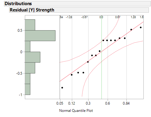
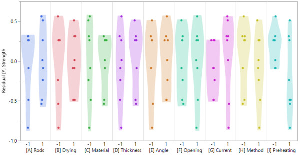
Der Normal-Quantil-Plot deutet nicht auf eine Verletzung der Normalverteilungsannahme hin. Betrachtet man die Scatterplots der einzelnen Faktoren gegenüber der Residuen, erkennt man dass die Annahme konstanter Varianzen nicht überall erfüllt ist. Für die Faktoren [B], [C], [G] and [I] scheint die Varianz der Residuen unterschiedlich in den verschiedenen Faktorstufen zu sein.
Abgesehen davon, dass damit eine unserer Annahmen der Regression verletzt ist und damit die resultierenden p-Werte nicht mehr verläßlich sind lernen wir hier schon etwas über unseren Prozess: Die erwähnten Faktoren scheinen einen Einfluß auf die Reproduzierbarkeit unserer Ergebnisse zu haben. Wirft man einen Blick auf Faktor [I], sieht man, dass der Prozess für die niedrige Einstellung (-1) recht robust zu sein scheint. Wählt man allerdings die hohe Einstellung (+1) sieht man eine hohe Streuung in den Daten. Das deutet auf eine geringe Reproduzierbarkeit der Ergebnisse hin.
Lösungsansätze
Es gibt eine Reihe von gängigen Empfehlungen zum Umgang mit Heteroskedastie in den Residuen:
- Variablentransformation: Eine Box-Cox-Power-Transformation kann hilfreich sein eine passende Transformation der Zielgröße zu finden. Oft erweist sich die Wurzel- oder Logarithmus-transformation als varianzstabilisierend.
- Verwendung andere Modelle: Verschiedene GLM-Ansätze (Verallgemeinerte Lineare Regression) erlauben nichtkonstante Varianz als Teil der Modellspezifikation.
- Heteroskedastie-Konsistente Standardfehler: White-Standard-Fehler berücksichtigen das Vorliegen von Heteroskedastie bei der Berechnung der Standardfehler der Regression und somit auch bei der Berechnung der p-Werte.
All diese Methoden haben eins gemeinsam: The versuchen das Problem von einem mathematischen Standpunkt aus zu lösen. Entweder man versucht die Heteroskedastie zu beseitigen (Transformation) oder als Teil der Modellspezifikation herauszurechnen.
Verwenden wir diese Methoden erhalten wir typischerweise keine tiefere Einsicht in die Ursachen der Heteroskedastie. Gerade wenn Robustheit ein zentraler Teil der Optimierung eines Prozesses ist, sind das keine passenden Lösungen.
Das loglinear Variance
Model Ein andere Ansatz wie man mit dem vorliegenden Problem umgehen kann sind die Loglinear Variance Models (In Ermangelung eines in der Wissenschaft verbreiteten Namens, benutze ich den Namen aus der JMP-Software für diese Modelle). Die Grundlegende Idee dieser Modelle ist es nicht nur den Mittelwert der Zielgrößen, sondern gleichzeitig auch die Varianz der Zielgröße zu modellieren. Während die einfache lineare Regression nur eine Mittelwertgleichung verwendet
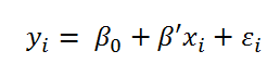
arbeiten Loglinear Variance Models mit den zwei folgenden Gleichungen:
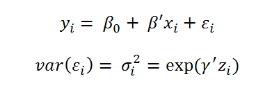
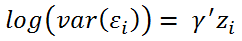
Offensichtlich wird hier der Logarithmus der Varianz mittels eines linearen Prädiktors beschreiben. Die Schätzung diese Modells ist natürlich etwas aufwändiger. Statt der Methode der einfachen kleinsten Quadrate wird hier ein REML-Ansatz benutzt. Das Vorgehen wird im Detail von [G. Smyth 2002] beschrieben.
Beispiel in JMP
Bevor wir uns mit den Ergebnissen des Modells und deren Interpretation beschäftigen muss man sich bewußt machen, dass es aufwändiger ist Varianzen zu schätzen als Mittelwerte. Demnach braucht man für die Schätzung von Loglinear Variance Models mehr Daten als bei der Verwendung von einfachen Regressionsmodellen. Im vorliegenden Fall heißt das, dass wir nicht in der Lage sind ein vollständiges Modell zu schätzen. D.h. ein Modell in dem alle Faktoren [A] bis [I] zur Beschreibung von Mittelwert und Varianz verwendet werden.
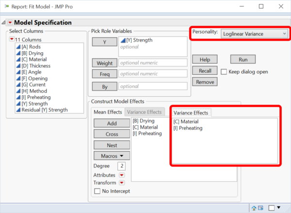
Für dieses Beispiel halten wir uns also an das von [Smyth 2002] vorgeschlagene Modell:
- Der Mittelwert wird beschrieben durch: [B], [C] und [I]
- Die Varianz wird beschrieben durch: [C] und [I]
In JMP 12 finden sich die Loglinear Variance Models in der Fit-Model-Plattform.
Die p-Werte im Abschnitt "Mean Model for [Y] Strength" zeigen uns, dass [B] und [C] einen statistisch signifikanten Einfluß auf die Reißfestigkeit haben. Faktor [I] ist nahe an der statistischen Signifikant zum Signifikanzniveau 5%.
Im Abschnitt "Variance Model for [Y] Strength" lernen wir, dass die Varianz der Residuen (=Reproduzierbarkeit des Prozesses) signifikant von den Faktoren [C] und [I] abhängt.
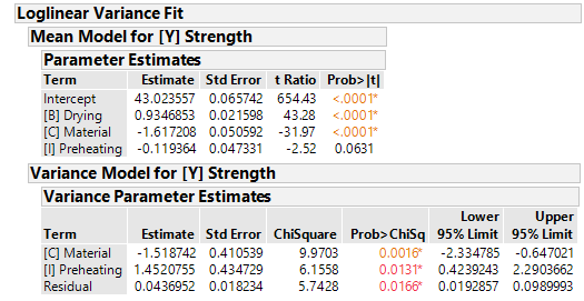
D.h. je nachdem mit welchen Stufen von [C] und [I] man Arbeitet ist der Prozess stabiler oder weniger stabil. Besonders der Einfluß von [I] - auf Mittelwert und Varianz - ist interessant, da der Faktor im einfachen Regressionsmodell komplett außen vor gelassen wurde.
Zur Optimierung können wir mit dem Analysediagramm in JMP arbeiten:
Die maximale Reißfestigkeit erreicht man mit hohen Settings von [B] und niedrigen Settings von [C]. Der Einfluß von [I] auf den Mittelwert ist eher marginal.
Gleichzeitig hat [C] einen negativen Einfluß auf die Varianz des Prozesses. D.h. für die Maximierung der Reißfestigkeit würden wir uns ein möglichst niedrige Werte von [C] wünschen. Für eine möglichst gute Reproduzierbarkeit sollte [C] aber auf einem hohen Level sein.
Einfacher ist es mit dem Faktor [I]. Der Einfluß auf den Mittelwert ist gering. Allerdings führen niedrige Settings von [I] zu deutlich geringere Varianz und sind somit vorzuziehen.
Schluss
- Loglineare Modell erlauben es gleichzeitig Mittelwert und Varianz zu modellieren. Damit eröffnen Sie komplett neue Möglichkeiten, besonders bei der Auswertung von DoEs.
- Ein Problem stellt allerdings dar, dass die klassischen DoEs nur darauf ausgelegt sind ein reines Mittelwertmodell zu schätzen. D.h. viele DoEs werden nicht genug Experimente zur Verfügung stellen um gleichzeitig ein sauberes Varianzmodell zu schätzen.
- Punkt 2 hat auch Auswirkung auf die Modellbildung, die generell noch nicht wirklich erforscht ist. Beim Thema Modellbildung können rein statistische Ansätze aber natürlich nie die Lösung sein. Hier wird immer Anwendungswissen benötigt werden.
Literatur und nützliche Quellen
- M. Aitkin: Modelling Variance Heterogeneity in Normal Regression using GLIM (Journal of Royal Statistical Society. Series C (Applied Statistics), 1987)
- H. Goldstein: Heteroscedasticity and Complex Variation (Encyclopedia of Statistics in Behavioral Science)
- A.C. Harvey: Estimating Regression Models with Multiplicative Heteroiscedasticity (Econometrica, 1976)
- G. Smyth: An Efficient Algorithm for REML in Heteroscedastic Regression (Journal of Computational and Graphical Statistics, 2002) JMP 12 Online Documentation